
QC Story – Control Charts
by: Quest Claire
Find this article helpful? Share it with others.

As I said in my first article, my direct supervisor Mr. Boss, VP Merchandising, asked me to present some recommendations to the company management to reduce customer returns from the annualized 8% to 6%.
Like many of our retail competitors, we are buying products from vendors with different levels of quality systems. Some of these vendors have a comprehensive quality system in place, i.e., ISO 9001 certified. However, many of them operate on a lean-and-mean quality system, just barely qualified to be suppliers of our company, Quality First.
These suppliers with lean and mean system need helps in maintaining their process capability, as a minimum, to manage process stability and control. I, therefore, plan to introduce the control chart statistical tool to them, expecting to help improve the outcome of their production and reduce the customer returns of Quality First. Upon understanding the constraints or limits of applying the control chart, I hope Quality First suppliers will be better positioned to determine if this statistical tool is helpful for their production processes.
Concept of the control charts
The ultimate objective of a process is to make the product conform to specifications. Once manufacturing planning and engineering provide production with capable processes, it is the role of process control to get the most out of these processes by running them at a stable and uniform level of performance. An important tool helping do this is the control chart.
A control chart is a graphic comparison of process performance data to compute quality control limits drawn as limit lines on the chart. The process performance data usually consist of groups of measurement (collected from subgroups) collected in a regular production sequence while preserving the order.

The prime use of the control chart is to detect assignable causes of variation in the process. The term assignable causes have a special meaning; it is essential to understand this meaning to understand the control chart concept.
Process variations are traceable to two kinds of causes, (1) random, for example, due solely to chances, and (2) assignable, for example, due to specific findable causes. These two types of process variation are also presented in the previous articles. When these variations fall beyond tolerable limits, defectives are produced. Categorically, the random causes have chronic defects, and the assignable causes produce sporadic defects.
Ideally, only random causes should be present in a process because this represents the minimum possible variation. A process operating without assignable causes of variation is said to be in a state of statistical control, usually abbreviated as “in control”. A process in control is not only doing the best possible production job, but the state of control also permits the realization of important fringe benefits of the types listed. Attainment of these basic and fringe benefits makes it so useful to identify and eliminate assignable causes of variation, which is the key function of a control chart.
The control chart distinguishes between random and assignable causes of variation by choosing the control limits. These are calculated from the loss of probability so that highly improbable random variations are presumed to be due not to random causes but to assignable causes. When the actual variation exceeds the control limits, it is a signal that assignable causes enter the process, and the process should be investigated. Variation within the control limits means that only random causes are present in the process, and the process should continue to run as designed.
Use of the control chart to detect assignable causes variation in the process takes two forms: (1) to determine whether an unknown process is in a state of control (this is called control with no standard given), (2) to determine whether a known process remains in a state of control (this is called control with standard given).
The steps needed to set up these two types of a control chart are quite similar. However, there are differences in the formulas for calculating the control limits, the symbols used for the statistics, and some of the concepts of significance.
For most control charts, the control limits are calculated based on the average +/- 3 times the standard deviation of the statistic used. Using +/- 3 times the standard deviation means that if random causes alone are present, 99.7% of the chart values will fall within the control limits. The remaining points, 0.3% become false alarms, but this frequency is so low that the +/-3s limits are often used to distinguish between random and assignable causes of variation. Conversely, a process outside statistical control may still produce a product that conforms to specifications. Actions on such a process usually have a much lower priority than actions on processes producing non-conforming products.
As I get into the details of constructing and using a control chart. What is the purpose behind doing it? The ultimate purpose of the process is to assure the product’s fitness for use at an optimum point of the production economy. Sometimes it is economical to keep a process in control as a better means of meeting the product specifications. It is sometimes economical to plot control charts to keep processes in control. However, using these means (charts, controlled processes) should be restricted to those situations where the means can economically aid the primary purpose of meeting product specifications. Considering the last number of quality characteristics in a modern plant, control charts are justified for only a small minority of the quality characteristics. Furthermore, once they have served their purpose (for problem analysis for breakthrough or control), most should be taken down, and the effort shifted to other characteristics needing improvement.

Steps in setting up control charts
a. Choose the characteristic to be charted. This is a matter of judgment but use the following guides.
1. Give high priority to characteristics that are currently running defective. These may be on basic or intermediate items such as parts, subassemblies, or products. A Pareto analysis can establish priorities.
2. Identify the process variables and conditions contributing to the product characteristics to define potential charting applications from raw material through processing steps to final characteristics.
3. Choose characteristics that will provide the data needed for problem diagnosis. Attributable data (percent effective) provide summary information but may need to be supplemented by variable data to diagnose causes and determine actions.
4. Determine the earliest point in the production process at which testing can be done to get information on assignable causes so that the chart can serve as an effective early warning device to prevent defectives.
b. Choose the type of control chart
c. Decide the center line to be used to calculate the control limits. The center line may be the average of past data or a desired average (i.e., the standard value). The limits are usually set at +/-3 standard deviations, but other multiples may be chosen for different statistical risks. For example, the +/-3 s limit involves a very small risk (usually less than 3 in 1,000) of looking for trouble that does not exist. However, these 3 limits may have a large risk of failing to detect trouble when it exists. Limits set at +/-2s would have a larger risk of the first type of error but a smaller risk of the second type. These risks depend on the sample size and other factors. Statistical studies found that charts using 2s or even 1.5s limits are more economical than conventional 3s limits. This is true if it is possible to decide very quickly and inexpensively that everything is fine with the process when a point (just by chance) happens to follow fall outside the control limits, i.e., when the cost is low of looking for trouble when none exists. Conversely, it will be more economical to use charts with 3.5s or 4s limits if the cost of looking for trouble is very high.
d. Choose the rational subgroup: the data chronologically plotted on a control chart consist of groups of a unit of product, and the groups are called rational subgroups. Subgroups should be chosen in a way that gives a maximum chance for the measurements in each subgroup to be alike and the maximum chance for the subgroups to differ from one another. The main point in choosing the rational subgroups is:
Lots from which the subgroups are chosen. The order of choice of the lot is a vital factor in determining whether a particular kind of variable is concealed or revealed. Any one lot should, so far as possible, have been made under like conditions so that the pieces in the lot are as alike as possible. The order of choice of the lots can be in one of several ways:
· By suspected causes of variation: in this case, each lot comprises products originating from a single ‘system of causes. For example, a six-spindle machine may be delivering product into a common delivery chute. To test whether any one of the spindles is a significant cause of variation, the product delivered by the six spindles should be kept segregated and would dare by separate constitutional lots. In like manner, the product of different operators, machines, shifts, material process conditions, etc., forms a natural basis for dividing the product into lots and subsequently choosing the subgroups from the segregated portions.
· Over each time interval: this is especially useful for disclosing causes that vary with time. Choices of lots over an equal interval are easy to organize and administer. Most control charts used for retaining control are on an equal time or quantity basis.
1. Composition and frequency of the subgroup:
When the chart is used for process control purposes, the pieces within each subgroup should be consecutively pieces in the order of production. This is desirable to obtain an estimate of chance variation, which will yield control limits sensitive enough to detect process change. Suppose the pieces are taken at random from a lot. In that case, the changes that occur as the lot progresses will increase the dispersion in the subgroup, resulting in wider control limits, thereby reducing the sensitivity of the chart.
The decision on the frequency of subgroups must balance the cost of taking subgroups against the value of data obtained.
Example:
Based on previous studies, if a shift in the process average causes a high rate of loss, i.e., high relative to the cost of inspection, it is better to take small group subgroups quite frequently than large subgroups less frequently. For example, when the loss rate is high, subgroups 4 or 5, taken every half hour, are better than subgroups of 8 or 10, taken every hour.
Suppose the unit cost of an inspection is relatively high. In that case, the most economical design takes small subgroups (say subgroup of 2) at relatively long intervals (say every 4 to 8 hours) with narrow control limits, say at +/- 1.5.
2. Subgroup size: the subgroup size decides the width of the limit lines and thereby decides the maximum extent of changes that will go undetected. The sensitivity of a chart for detecting process changes of varying degrees with different subgroup sizes can be defined by an operating characteristic curve.
a. Provide a system for collecting the data
If the control chart is to serve as a day-to-day shop tool, it must be made simple and convenient for use. Measurement must be simplified and kept free of error. Indicating instruments must be designed to give prompt and reliable readings. Better yet, instruments should be designed to record and display. Data recording can be simplified by the skillful design of data or tally sheets. The working conditions are a factor. A machine department that abounds in cutting oil cannot keep respectable records with ordinary pencil and paper. Protective cover, special paper and crayons can be provided. Copies of day-to-day data should be avoided.
b. Calculate the control limits and provide specific instructions on interpreting the results and the actions to be taken by various production personnel.

P Control Charts
This type of control chart is useful for consumer product production, in which acceptance of quality is solely based on if a product is non-defective. p control charts monitor variation in go/no-go type attributes data. There are only two possible outcomes: the item is defective or non-defective. The p control chart determines if the fraction of defective items in a group of items is statistically stable over time.
A product is defective if it fails to conform to specifications or standards. For example, consider the case of a toy factory producing toys for a client like Quality First. Quality First wants the product quality to be under 2.5% defective. Using this definition, we monitor the defective toy regularly and ensure this requirement is met.
I recommend that our toy factory use a p control chart to monitor defective and non-defective data. This type of chart involves counts. In counting items for using a p control chart, the counts must also satisfy the following two conditions:
- In counting n items, the count is the number of items in those n items that is defective.
- Suppose p is the probability that an item is defective; the value of p must be the same for each of the n items in a single sample.
If these two conditions are met, the binomial distribution can be used to estimate the distribution of the counts and the p control chart can be used. Care must be taken because condition 2 may not always hold. For example, some people use the p control chart to monitor on-time delivery every month. This is only valid if the probability of each shipment during the month being on time is the same for all the shipments. Big customers often get priority on their orders, so the probability of their orders being on time is different from that of other customers. In that case, the p control chart should not be used. The example below will take you through constructing a p control chart.
An example for illustration purposes:
The Paint Spraying Process inspection from a toy factory has been working on improving the processing of the paint spraying process. The factory management is trying to reduce the quality cost of the spraying process by decreasing the percentage of painting discrepancies (collectively named defectives which contain major defectives, minor defectives, and certain tolerable discrepancies). The management developed the following operational definition for painting discrepancies: if the toy contains paint with blurred paint, over/under painting, smeared paint, and a few other similar types of defects. The inspection team decided to pull a random sample of 100 toys per day. If a toy contains one or more discrepancies, it is defective. The data from 4 weeks, a total of 25 days, are given in the table.
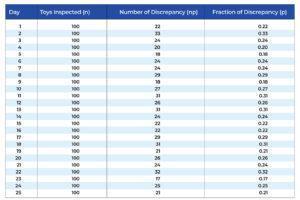
These data will be used to construct a p control chart. The subgroup size is n = 100. The p values for each subgroup (each day) are calculated and shown in the table. For example, on day 1, 22 discrepant items (np) were found in the 100 toys inspected. Thus, p = np/n = 22/100 = 0.22 or 22%. The p values for the other days are calculated similarly.
Average and Control Limits:
The next step is to calculate the average fraction discrepancy. To determine the average, we add all the np values and divide them by the sum of all the n values. The sum of the np values is 621; the sum of the n values is 2500. The average is then calculated as shown below.
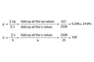
The next step is to determine the average subgroup size. Since the subgroup size is constant, the average subgroup size is 100. The second equation shows this average calculation, where k is the number of subgroups. The next step is to calculate the control limits. The control limits calculations are shown below.
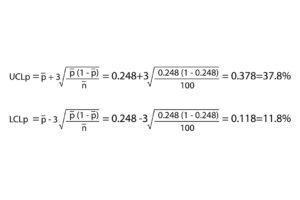
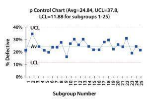
Making use of these data and calculated values, the p control chart is constructed as follows:
The following questions and answers, as related to the p control chart, are meant to help interpret the p control chart generated:
- What variation is the p control chart examining?
The variation being examined is the variation in the percentage of discrepancy of spray painting from day to day.
- Is the process in statistical control? What does this mean?
The process is in statistical control. This means that the process is consistent and predictable. On average, each day will have about 25% of the toys containing painting discrepancies. Some days it may be as high as 37% or as low as 12%. Only non-assignable causes of variation are present. The process is in statistical control.
- What should be done next to work on improving this process?
Note that this does not mean that the process is acceptable. Having 25% of paint spraying discrepancies is not acceptable. The next step is to apply a troubleshooting process to identify the non-assignable causes of the chronic problems to reduce the number of discrepancies.
4. What could another type of statistical tool be used in conjunction with this p control chart and why?
A Pareto diagram supported by the remedial process is an effective tool along with the use of this p control chart. The Pareto diagram determines the reason for defects and the frequency with which they occur, as discussed in the previous articles.
An important message for using Varying Subgroup Sizes:
In constructing a p control chart, the subgroup size should be constant. If not, the values of n should not vary by more than ± 25%. The impact of the subgroup size can be seen by examining the equations for the control limits. The control limits have the average subgroup size in the denominator under the square root sign. If the subgroup size varies too much, the average subgroup size is not a good estimator of n. Therefore, the control limits must be calculated for each varying subgroup size in these cases. In the control limit equations, nbar is replaced by n, the actual subgroup size.
Before closing this article, I like to remind you that the purpose of developing these articles is to help the suppliers operating based on basic lean and mean systems just to be qualified for doing business with Quality First. These suppliers may or may not be staffed with the necessary Production or QC personnel to enforce the discussed process capability improvement. Any further actions to expand their company’s technical capability and expertise, to solidify their commitment to beefing up their capability for getting future business will remain their individual management decision.